Exam prep · AP Statistics · Unit guide
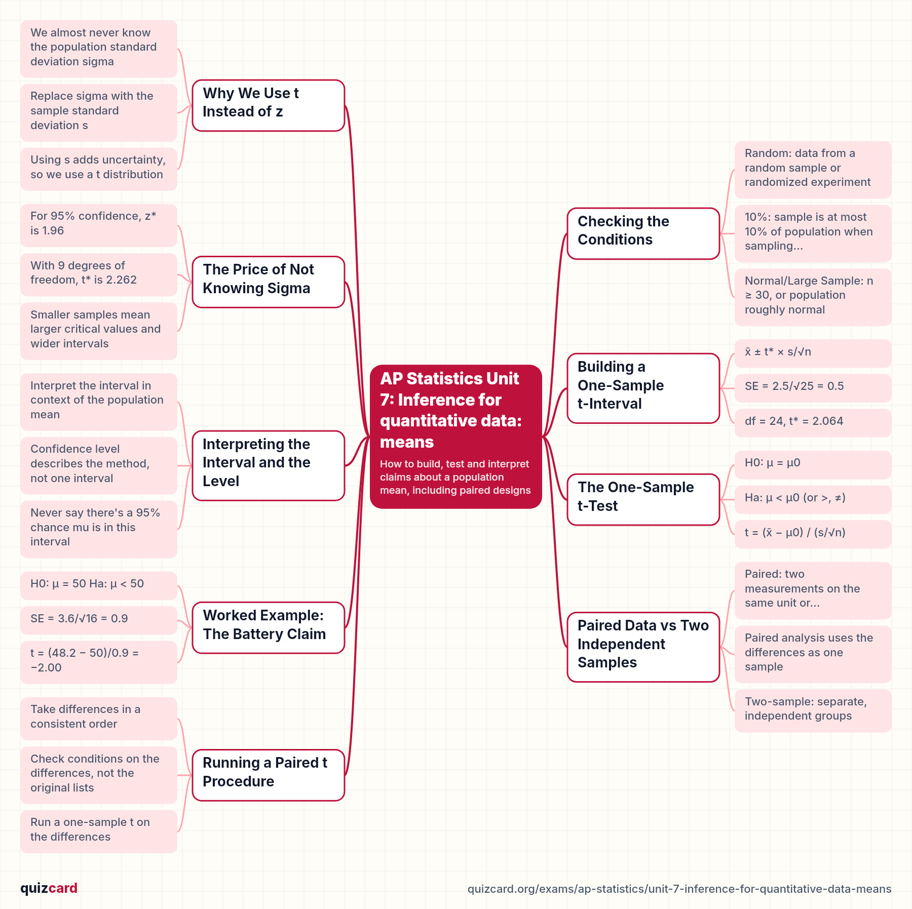
AP Statistics Unit 7: Inference for quantitative data: means
How to build, test and interpret claims about a population mean, including paired designs
On the exam: t-intervals and t-tests, paired data. 10 to 18%.
Quick check: if the same twenty students take a test before and after tutoring, are those two independent samples? Most people say yes, and that's wrong. In this video for your statistics course, we'll cover t-intervals, t-tests, conditions, a worked problem, and paired data.
Why We Use t Instead of z
When you estimate a population mean, you almost never know the population standard deviation, so you plug in the sample standard deviation, s, instead. That substitution adds extra uncertainty, and the t distribution accounts for it. It's centered at zero and symmetric like the normal curve, but its tails are heavier. How heavy depends on the degrees of freedom, which is n minus one for one sample. As degrees of freedom grow, t gets closer and closer to z.
z procedures
- Population SD sigma is known
- Standard normal curve
- No degrees of freedom
- Used for proportions in practice
t procedures
- Sigma unknown, use sample SD s
- Heavier tails than normal
- Shape set by df = n − 1
- Approaches z as df grows
Checking the Conditions
Before any t procedure, you check three conditions. First, the data must come from a random sample or a randomized experiment. Second, if you sample without replacement, the sample should be no more than ten percent of the population, so observations are roughly independent. Third, the sampling distribution of the mean must be approximately normal. That's fine if n is at least thirty, or if a dotplot or boxplot of a small sample shows no strong skew or outliers.
Key points.
- Random: data from a random sample or randomized experiment
- 10%: sample is at most 10% of population when sampling without replacement
- Normal/Large Sample: n ≥ 30, or population roughly normal
- For small n, graph the data: no strong skew or outliers
The Price of Not Knowing Sigma
Here's what those heavier tails do in practice. For ninety-five percent confidence, the critical value z star is one point nine six. But with a sample of ten, which gives nine degrees of freedom, the critical value t star jumps to two point two six two. That larger multiplier makes the interval wider, which is the honest cost of estimating the spread from a small sample. You find t star from a t table or with your calculator's inverse t function.
2.262 t* for 95% confidence with df = 9, compared with z* = 1.96
Key points.
- For 95% confidence, z* is 1.96
- With 9 degrees of freedom, t* is 2.262
- Smaller samples mean larger critical values and wider intervals
Building a One-Sample t-Interval
The interval is the sample mean plus or minus t star times the standard error. The standard error is s divided by the square root of n. Say n is twenty-five, the sample mean is twelve point four, and s is two point five. The standard error is two point five over five, which is zero point five. With twenty-four degrees of freedom, t star is two point zero six four, so the margin is one point zero three two, giving about eleven point three seven to thirteen point four three.
x̄ ± t* × s/√n
SE = 2.5/√25 = 0.5
df = 24, t* = 2.064
12.4 ± 2.064 × 0.5
12.4 ± 1.032
(11.37, 13.43)
Key points.
- Interval is point estimate plus or minus margin of error
- Standard error of the mean is s divided by root n
- Example: n = 25, mean 12.4, s = 2.5 gives (11.37, 13.43)
Interpreting the Interval and the Level
Graders look for a specific interpretation. You say you're ninety-five percent confident that the interval captures the true population mean, and you name that mean in context. The confidence level itself is about the method. If you took many random samples and built an interval from each, about ninety-five percent of them would capture the true mean. Avoid saying there's a ninety-five percent probability that this particular interval contains it.
We are 95% confident that the interval from 11.37 to 13.43 captures the true mean of the population, in context. Standard interpretation template
Key points.
- Interpret the interval in context of the population mean
- Confidence level describes the method, not one interval
- Never say there's a 95% chance mu is in this interval
The One-Sample t-Test
A significance test starts with hypotheses about the population mean. The null says mu equals some claimed value, mu naught, and the alternative says it's less, greater, or not equal. The test statistic is the sample mean minus mu naught, divided by s over root n. You use n minus one degrees of freedom, and the p-value is the probability of a t value at least as extreme as yours, assuming the null is true.
H0: μ = μ0
Ha: μ < μ0 (or >, ≠)
t = (x̄ − μ0) / (s/√n)
df = n − 1
p = P(t ≤ observed | H0)
Key points.
- Hypotheses are about the population mean mu
- Test statistic: (x̄ − μ0) divided by s/√n
- p-value comes from the t distribution with n − 1 df
- Small p-value is convincing evidence for Ha
Worked Example: The Battery Claim
A company claims its batteries last fifty hours on average. A random sample of sixteen lasts a mean of forty-eight point two hours with s of three point six. Is there convincing evidence the true mean is less? The null is mu equals fifty, the alternative is less than fifty. The standard error is three point six over four, which is zero point nine. So t equals negative one point eight over zero point nine, which is negative two, with fifteen degrees of freedom. The p-value is about zero point zero three two, below zero point zero five, so we reject the null.
H0: μ = 50   Ha: μ < 50
SE = 3.6/√16 = 0.9
t = (48.2 − 50)/0.9 = −2.00
df = 15,  p ≈ 0.032
0.032 < 0.05 → reject H0
Key points.
- Claim: mean battery life is 50 hours
- Random sample: n = 16, mean 48.2, s = 3.6
- t = −2.00, df = 15, p ≈ 0.032
- Reject H0 at 0.05: convincing evidence mean is below 50
Paired Data vs Two Independent Samples
Now back to the tutoring trap from the start. When each student is measured before and after, the two lists are linked, so the data are paired. You don't compare two means; you compute one difference per student and analyze those differences. Two-sample t procedures are for truly separate groups, like a random sample of men and another of women. Their standard error is the square root of s one squared over n one plus s two squared over n two.
Paired t
- Same subjects measured twice, or matched pairs
- Analyze differences, mean μd
- SE = sd/√n, df = n − 1
- Pre-test and post-test on same students
Two-sample t
- Two independent random samples or groups
- Parameter is μ1 − μ2
- SE = √(s1²/n1 + s2²/n2)
- df from calculator, or smaller n − 1
Running a Paired t Procedure
Here's the paired routine. First, subtract in a consistent order, such as after minus before, for every pair. Then check the conditions on those differences: random, ten percent, and either n of at least thirty or a graph of the differences with no strong skew or outliers. Next, find the mean and standard deviation of the differences and run a one-sample t procedure with n minus one degrees of freedom. Finally, state your conclusion about the true mean difference in context.
- Compute each difference (after − before)
- Check conditions on the differences
- Find mean and SD of the differences
- Run one-sample t on differences, df = n − 1
- Conclude about μd in context
Remember this
If you remember one thing, make it this: decide first whether your data are one sample, paired, or two independent groups, because everything else follows from that. Now try quizzing yourself on a few practice problems.
Practice this unit
- Statistics 101: Core Concepts30 flashcards · study free
- Statistics: Hypothesis Testing Practice30 flashcards · study free
- AP Statistics: Probability, Random Variables and Sampling Distributions38 flashcards · study free
Every AP Statistics deck and quiz: the AP Statistics hub.
Other AP Statistics unit guides
Try it with your own material
Upload a PDF, slides or notes and study the deck in minutes. Making your own cards is free with no limits.