Exam prep · AP Statistics · Unit guide
AP Statistics Unit 5: Sampling distributions
How sample proportions and sample means vary, and when you can treat them as normal
On the exam: Central limit theorem, distributions of sample means and proportions. 7 to 12%.
Quick question: if you take a bigger sample, does your data start looking normal? Most students say yes, and that's the mistake. In this video for your stats exam, we'll cover sampling distributions, proportions, means, the Central Limit Theorem, and a full worked problem.
What a Sampling Distribution Is
Let's start with vocabulary. A parameter is a number that describes a population, like the true proportion p or the true mean mu. A statistic is a number from a sample, like p hat or x bar. Because every random sample is different, a statistic varies from sample to sample. The sampling distribution captures that variation across all possible samples of the same size.
The distribution of values taken by a statistic in all possible samples of the same size from the same population. Standard definition
Key points.
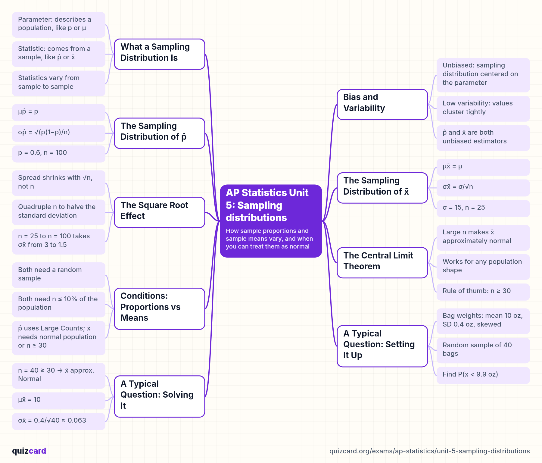
- Parameter: describes a population, like p or μ
- Statistic: comes from a sample, like p̂ or x̄
- Statistics vary from sample to sample
- Sampling distribution: all possible values of a statistic
Bias and Variability
A statistic is an unbiased estimator when the mean of its sampling distribution equals the parameter it estimates. Picture a dartboard where the bullseye is the parameter. Unbiased means the darts center on the bullseye, and low variability means they cluster tightly. Sample proportions and sample means are both unbiased, and their variability shrinks as the sample size grows, not as the population grows.
Key points.
- Unbiased: sampling distribution centered on the parameter
- Low variability: values cluster tightly
- p̂ and x̄ are both unbiased estimators
- Larger samples mean less variability
The Sampling Distribution of p̂
For a sample proportion, the mean of the sampling distribution is p. The standard deviation is the square root of p times one minus p, over n. With p equal to point six and n equal to one hundred, that's the square root of point two four over one hundred, about point zero four nine. Since n p is sixty and n times one minus p is forty, both at least ten, the shape is approximately normal.
μp̂ = p
σp̂ = √(p(1−p)/n)
p = 0.6, n = 100
σp̂ = √(0.24/100) ≈ 0.049
np = 60 ≥ 10, n(1−p) = 40 ≥ 10
Key points.
- Mean of p̂ equals p
- Standard deviation is √(p(1−p)/n)
- Normal shape if np ≥ 10 and n(1−p) ≥ 10
The Sampling Distribution of x̄
For a sample mean, the center of the sampling distribution equals the population mean, mu. The spread is sigma over the square root of n. Suppose test scores have a standard deviation of fifteen and you take samples of twenty-five. Then the standard deviation of x bar is fifteen over the square root of twenty-five, which is fifteen over five, or three. Averages vary much less than individuals do.
μx̄ = μ
σx̄ = σ/√n
σ = 15, n = 25
σx̄ = 15/√25 = 15/5 = 3
Key points.
- Mean of x̄ equals μ
- Standard deviation of x̄ is σ/√n
- Averages vary less than individual values
The Square Root Effect
Here's a detail that shows up again and again. Because n sits under a square root, the spread doesn't shrink in proportion to the sample size. To cut the standard deviation in half, you need four times as many observations. Going from twenty-five to one hundred takes our test score example from a standard deviation of three down to one and a half, not down to three quarters.
4× Sample size needed to cut a statistic's standard deviation in half
Key points.
- Spread shrinks with √n, not n
- Quadruple n to halve the standard deviation
- n = 25 to n = 100 takes σx̄ from 3 to 1.5
The Central Limit Theorem
The Central Limit Theorem says that when n is large, the sampling distribution of x bar is approximately normal, no matter what shape the population has. Picture a strongly right-skewed population, like household incomes. Take many samples of size thirty and plot each mean, and the histogram of those means looks close to a bell curve. If the population itself is normal, x bar is normal for any sample size.
Key points.
- Large n makes x̄ approximately normal
- Works for any population shape
- Rule of thumb: n ≥ 30
- Normal population gives normal x̄ for any n
Conditions: Proportions vs Means
Let's line up the conditions side by side, because mixing them up is easy. Both statistics need a random sample, and both need the ten percent condition, so the sample is at most a tenth of the population. For shape, proportions use the Large Counts condition, while means need either a normal population or n of at least thirty. Remember, the Central Limit Theorem describes the sampling distribution, never the sample data itself.
Sample proportion p̂
- Random sample
- 10%: n ≤ 0.10 × population
- Large Counts: np ≥ 10 and n(1−p) ≥ 10
Sample mean x̄
- Random sample
- 10%: n ≤ 0.10 × population
- Normal population, or n ≥ 30 (CLT)
A Typical Question: Setting It Up
Now let's try a typical question. Bag weights of chips are skewed, with a mean of ten ounces and a standard deviation of point four ounces. If you randomly sample forty bags, what's the probability their mean weight is below nine point nine ounces? Work it in four moves: name the statistic, check the conditions, find its mean and standard deviation, then standardize and answer in context.
- Name the statistic: the sample mean x̄
- Check random, 10%, and n ≥ 30
- Find the mean and SD of x̄
- Compute z, find the probability, answer in context
A Typical Question: Solving It
Since n is forty, which is at least thirty, the Central Limit Theorem says x bar is approximately normal. Its mean is ten, and its standard deviation is point four over the square root of forty, about point zero six three. The z-score is nine point nine minus ten, over point zero six three, about negative one point five eight. So the probability is about point zero five seven, roughly a six percent chance.
n = 40 ≥ 30 → x̄ approx. Normal
μx̄ = 10
σx̄ = 0.4/√40 ≈ 0.063
z = (9.9 − 10)/0.063 ≈ −1.58
P(x̄ < 9.9) ≈ 0.057
Key points.
- n = 40 ≥ 30, so x̄ is approximately normal
- σx̄ = 0.4/√40 ≈ 0.063
- z ≈ −1.58, probability ≈ 0.057
Remember this
Remember this: a sampling distribution shows how a statistic varies from sample to sample, and its spread shrinks with the square root of n. Now quiz yourself on the formulas and conditions to see what sticks.
Practice this unit
- Statistics 101: Core Concepts30 flashcards · study free
- Statistics: Hypothesis Testing Practice30 flashcards · study free
- AP Statistics: Probability, Random Variables and Sampling Distributions38 flashcards · study free
Every AP Statistics deck and quiz: the AP Statistics hub.
Other AP Statistics unit guides
Try it with your own material
Upload a PDF, slides or notes and study the deck in minutes. Making your own cards is free with no limits.